Based on https://satijalab.org/seurat/articles/integration_introduction.html
suppressWarnings(library(Seurat))
## Registered S3 method overwritten by 'spatstat.geom':
##   method     from
##   print.boxx cli

## Attaching SeuratObject
suppressWarnings(library(SeuratData))
## -- Installed datasets ------------------------------------- SeuratData v0.2.1 --

## v ifnb   3.1.0                          v pbmc3k 3.1.4

## -------------------------------------- Key -------------------------------------

## v Dataset loaded successfully
## > Dataset built with a newer version of Seurat than installed
## (?) Unknown version of Seurat installed
suppressWarnings(library(patchwork))
Chapter 1 - Build an merged Seurat Object using own data
You can also load your own data using the read10x function Make sure you have all three file in the correct directory
- matrix.mtx
- genes.tsv
- barcodes.tsv
URL <- "D:/Documents/GitHub/Introduction-to-Seurat-Package/pbmc3k_filtered_gene_bc_matrices/filtered_gene_bc_matrices/hg19"

# Load the PBMC dataset1
pbmc.data1 <- Read10X(data.dir = URL)
# Initialize the Seurat object with the raw (non-normalized data).
ctrl <- CreateSeuratObject(counts = pbmc.data1, project = "pbmc3k", min.cells = 300, min.features = 200)

# Load the PBMC dataset2
pbmc.data2 <- Read10X(data.dir = URL)
# Initialize the Seurat object with the raw (non-normalized data).
stim <- CreateSeuratObject(counts = pbmc.data2, project = "pbmc3k", min.cells = 600, min.features = 200)

pmbc.list <- list(ctrl,stim)
merged.pbmc <- merge(x = ctrl, y = stim, add.cell.ids = c("3K", "4K"))

#more than one sample
#merged.pbmc <- merge(x = ctrl, y = c(stim1,stim2,stim3))

#Example from seurat
#https://satijalab.org/seurat/articles/merge_vignette.html
#pbmc.big <- merge(pbmc3k, y = c(pbmc4k, pbmc8k), add.cell.ids = c("3K", "4K", "8K"), project = "PBMC15K")
#pbmc.big
Chapter 1 - Adding MetaData
library(stringr)
sample <- names(merged.pbmc@active.ident)
sample_detect <- ifelse(str_detect(sample,"3K"),"3K","4K")

merged.pbmc@meta.data$sample <- sample_detect

Idents(object = merged.pbmc) <- "sample"
Chapter 1 - Normalized Data and Intergrate the two dataset
pmbc.list <-  SplitObject(merged.pbmc, split.by = "sample")

# perform standard preprocessing on each object
for (i in 1:length(pmbc.list)) {
  pmbc.list[[i]] <- NormalizeData(pmbc.list[[i]], verbose = FALSE)
  pmbc.list[[i]] <- subset(pmbc.list[[i]], downsample = 1000)
  pmbc.list[[i]] <- FindVariableFeatures(
    pmbc.list[[i]], selection.method = "vst",
    nfeatures = 2000, verbose = FALSE
  )
}

# select features that are repeatedly variable across datasets for integration run PCA on each
# dataset using these features
features <- SelectIntegrationFeatures(object.list = pmbc.list)
pmbc.list <- lapply(X = pmbc.list, FUN = function(x) {
    x <- ScaleData(x, features = features, verbose = FALSE)
    x <- RunPCA(x, features = features, verbose = FALSE)
})
Chapter 1 - Intergrate Data
#####################
# find anchors
anchors <- FindIntegrationAnchors(object.list = pmbc.list)
## Computing 2000 integration features

## Scaling features for provided objects

## Finding all pairwise anchors

## Running CCA

## Merging objects

## Finding neighborhoods

## Finding anchors

##  Found 3803 anchors

## Filtering anchors

##  Retained 3018 anchors
# integrate data
merged.pbmc <- IntegrateData(anchorset = anchors)
## Merging dataset 2 into 1

## Extracting anchors for merged samples

## Finding integration vectors

## Finding integration vector weights

## Integrating data
Chapter 1.2 - Data Cleaning and Dimensional reduction for visualization
# Run the standard workflow for visualization and clustering
merged.pbmc <- ScaleData(merged.pbmc, verbose = FALSE)
merged.pbmc <- FindVariableFeatures(merged.pbmc,
                                    selection.method = "vst",
                                    nfeatures = 2000,
                                    verbose = FALSE)
## Warning in FindVariableFeatures.Assay(object = assay.data, selection.method =
## selection.method, : selection.method set to 'vst' but count slot is empty; will
## use data slot instead
merged.pbmc <- RunPCA(merged.pbmc, npcs = 30, verbose = FALSE)
merged.pbmc <- RunUMAP(merged.pbmc, reduction = "pca", dims = 1:30)
## Warning: The default method for RunUMAP has changed from calling Python UMAP via reticulate to the R-native UWOT using the cosine metric
## To use Python UMAP via reticulate, set umap.method to 'umap-learn' and metric to 'correlation'
## This message will be shown once per session

## 13:14:12 UMAP embedding parameters a = 0.9922 b = 1.112

## 13:14:12 Read 2000 rows and found 30 numeric columns

## 13:14:12 Using Annoy for neighbor search, n_neighbors = 30

## 13:14:12 Building Annoy index with metric = cosine, n_trees = 50

## 0%   10   20   30   40   50   60   70   80   90   100%

## [----|----|----|----|----|----|----|----|----|----|

## **************************************************|
## 13:14:13 Writing NN index file to temp file C:\Users\harpa\AppData\Local\Temp\RtmpQV6obQ\file3b945fe1326e
## 13:14:13 Searching Annoy index using 1 thread, search_k = 3000
## 13:14:13 Annoy recall = 100%
## 13:14:14 Commencing smooth kNN distance calibration using 1 thread
## 13:14:14 Initializing from normalized Laplacian + noise
## 13:14:14 Commencing optimization for 500 epochs, with 90866 positive edges
## 13:14:23 Optimization finished
merged.pbmc <- FindNeighbors(merged.pbmc, reduction = "pca", dims = 1:30)
## Computing nearest neighbor graph
## Computing SNN
merged.pbmc <- FindClusters(merged.pbmc, resolution = 0.5)
## Modularity Optimizer version 1.3.0 by Ludo Waltman and Nees Jan van Eck
##
## Number of nodes: 2000
## Number of edges: 113355
##
## Running Louvain algorithm...
## Maximum modularity in 10 random starts: 0.8722
## Number of communities: 9
## Elapsed time: 0 seconds
gc()
##            used  (Mb) gc trigger  (Mb) max used  (Mb)
## Ncells  2768169 147.9    5367582 286.7  5367582 286.7
## Vcells 37097706 283.1   84887931 647.7 82907491 632.6
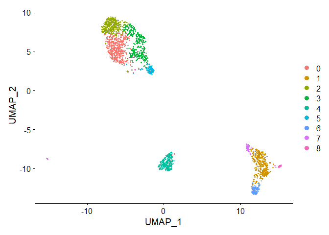
# Visualization

p1 <- DimPlot(merged.pbmc, reduction = "umap")
p1
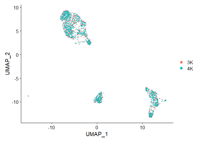
Idents(object = merged.pbmc) <- "sample"
p2 <- DimPlot(merged.pbmc, reduction = "umap")
p2
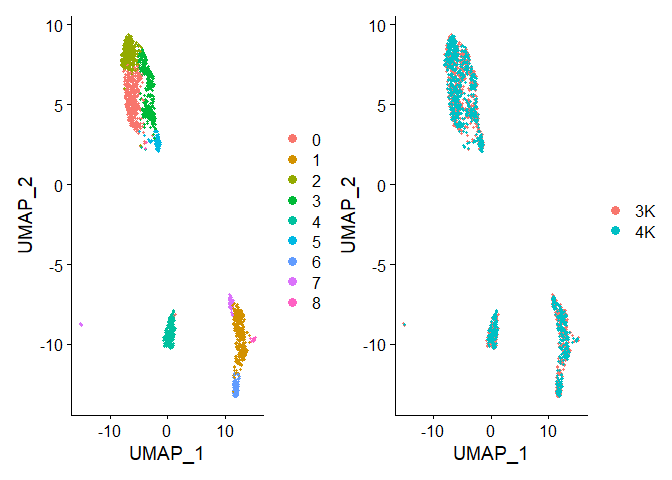
p1+p2
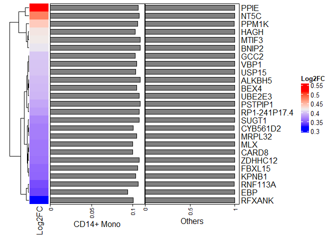
# Find differentially expressed features between CD14+ Monocytes and all other cells, only
# search for positive markers
Idents(object = merged.pbmc) <- "sample"

sammple.markers <- FindMarkers(merged.pbmc, ident.1 = "3K", ident.2 = "4K")
# view results
head(sammple.markers)
##                  p_val avg_log2FC pct.1 pct.2     p_val_adj
## EBP      1.504473e-238  0.3406139 0.094 0.999 2.846463e-235
## MLX      1.389999e-231  0.3645216 0.100 1.000 2.629877e-228
## CARD8    1.389999e-231  0.3642012 0.100 1.000 2.629878e-228
## RFXANK   1.300650e-228  0.3218905 0.101 0.996 2.460830e-225
## CYB561D2 3.550510e-228  0.3677264 0.101 0.995 6.717564e-225
## HAGH     6.276764e-228  0.4230465 0.103 1.000 1.187564e-224
# There shouldn't be any, but.........

library(ComplexHeatmap)
## Loading required package: grid

## ========================================
## ComplexHeatmap version 2.11.1
## Bioconductor page: http://bioconductor.org/packages/ComplexHeatmap/
## Github page: https://github.com/jokergoo/ComplexHeatmap
## Documentation: http://jokergoo.github.io/ComplexHeatmap-reference
##
## If you use it in published research, please cite:
## Gu, Z. Complex heatmaps reveal patterns and correlations in multidimensional
##   genomic data. Bioinformatics 2016.
##
## The new InteractiveComplexHeatmap package can directly export static
## complex heatmaps into an interactive Shiny app with zero effort. Have a try!
##
## This message can be suppressed by:
##   suppressPackageStartupMessages(library(ComplexHeatmap))
## ========================================
heatmapdf <- sammple.markers[1:25,]
row_ha = rowAnnotation("CD14+ Mono" = anno_barplot(heatmapdf$pct.1),
                       "Others"= anno_barplot(heatmapdf$pct.2),
                       width = unit(10, "cm"))

ht0 <- Heatmap(heatmapdf$avg_log2FC,
                name = "Log2FC",
                cluster_rows = TRUE,
                row_labels = rownames(heatmapdf),
                right_annotation = row_ha,
                width = unit(1, "cm"))

ht0
# Find differentially expressed features between CD14+ Monocytes and all other cells, only
# search for positive markers
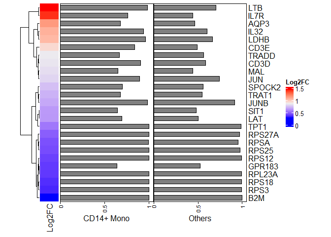
Idents(object = merged.pbmc) <- "seurat_clusters"

cluster1.de.markers <- FindMarkers(merged.pbmc, ident.1 = "0", ident.2 = NULL, only.pos = TRUE)
# view results
head(cluster1.de.markers)
##             p_val avg_log2FC pct.1 pct.2    p_val_adj
## LTB  2.122043e-87  1.4506039 0.983 0.700 4.014906e-84
## LDHB 5.833112e-72  1.0527473 0.961 0.664 1.103625e-68
## IL32 1.055335e-70  1.0788059 0.939 0.601 1.996693e-67
## TPT1 2.409722e-52  0.5544837 1.000 0.985 4.559194e-49
## AQP3 2.515788e-52  1.1517965 0.678 0.463 4.759870e-49
## IL7R 3.722894e-51  1.4124211 0.763 0.442 7.043715e-48
library(ComplexHeatmap)

heatmapdf <- cluster1.de.markers[1:25,]
row_ha = rowAnnotation("CD14+ Mono" = anno_barplot(heatmapdf$pct.1),
                       "Others"= anno_barplot(heatmapdf$pct.2),
                       width = unit(10, "cm"))

ht1 <- Heatmap(heatmapdf$avg_log2FC,
                name = "Log2FC",
                cluster_rows = TRUE,
                row_labels = rownames(heatmapdf),
                right_annotation = row_ha,
                width = unit(1, "cm"))

ht1
####################################################################
Chapter 2 - Using ifnb Dataset (The proper way)
# install dataset for the first time
#InstallData("ifnb")

# load dataset
suppressWarnings(suppressMessages(LoadData("ifnb")))
## An object of class Seurat
## 14053 features across 13999 samples within 1 assay
## Active assay: RNA (14053 features, 0 variable features)
ifnb <- ifnb

#?ifnb
# split the dataset into a list of two seurat objects (stim and CTRL)
ifnb.list <- SplitObject(ifnb, split.by = "stim")
ifnb.list <- lapply(X = ifnb.list, FUN = NormalizeData)

# normalize and identify variable features for each dataset independently
ifnb.list <- lapply(X = ifnb.list, FUN = function(x) {
    x <- subset(x, downsample = 1000)
    x <- FindVariableFeatures(x, selection.method = "vst", nfeatures = 2000)

})
Chapter 2 - Feature selection
# select features that are repeatedly variable across datasets for integration
features <- SelectIntegrationFeatures(object.list = ifnb.list)
immune.anchors <- FindIntegrationAnchors(object.list = ifnb.list, anchor.features = features)
## Scaling features for provided objects

## Finding all pairwise anchors

## Running CCA

## Merging objects

## Finding neighborhoods

## Finding anchors

##  Found 3188 anchors

## Filtering anchors

##  Retained 2460 anchors
# this command creates an 'integrated' data assay
immune.combined <- IntegrateData(anchorset = immune.anchors)
## Merging dataset 2 into 1

## Extracting anchors for merged samples

## Finding integration vectors

## Finding integration vector weights

## Integrating data
Chapter 2 - Data Procecssing
# specify that we will perform downstream analysis on the corrected data note that the
# original unmodified data still resides in the 'RNA' assay
DefaultAssay(immune.combined) <- "integrated"

# Run the standard workflow for visualization and clustering
immune.combined <- ScaleData(immune.combined, verbose = FALSE)
immune.combined <- RunPCA(immune.combined, npcs = 30, verbose = FALSE)
immune.combined <- RunUMAP(immune.combined, reduction = "pca", dims = 1:30)
## 13:15:24 UMAP embedding parameters a = 0.9922 b = 1.112

## 13:15:24 Read 2000 rows and found 30 numeric columns

## 13:15:24 Using Annoy for neighbor search, n_neighbors = 30

## 13:15:24 Building Annoy index with metric = cosine, n_trees = 50

## 0%   10   20   30   40   50   60   70   80   90   100%

## [----|----|----|----|----|----|----|----|----|----|

## **************************************************|
## 13:15:25 Writing NN index file to temp file C:\Users\harpa\AppData\Local\Temp\RtmpQV6obQ\file3b94734c3976
## 13:15:25 Searching Annoy index using 1 thread, search_k = 3000
## 13:15:25 Annoy recall = 100%
## 13:15:26 Commencing smooth kNN distance calibration using 1 thread
## 13:15:27 Initializing from normalized Laplacian + noise
## 13:15:27 Commencing optimization for 500 epochs, with 84996 positive edges
## 13:15:36 Optimization finished
immune.combined <- FindNeighbors(immune.combined, reduction = "pca", dims = 1:30)
## Computing nearest neighbor graph
## Computing SNN
immune.combined <- FindClusters(immune.combined, resolution = 0.5)
## Modularity Optimizer version 1.3.0 by Ludo Waltman and Nees Jan van Eck
##
## Number of nodes: 2000
## Number of edges: 102425
##
## Running Louvain algorithm...
## Maximum modularity in 10 random starts: 0.8758
## Number of communities: 10
## Elapsed time: 0 seconds
gc()
##            used  (Mb) gc trigger   (Mb)  max used   (Mb)
## Ncells  4634480 247.6    9451438  504.8   9451438  504.8
## Vcells 89072648 679.6  184431107 1407.1 184430469 1407.1
Chapter 2 - Visualise Data
# Visualization
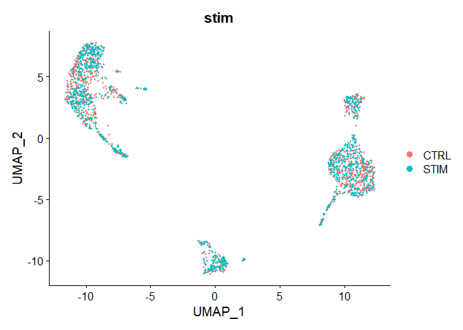
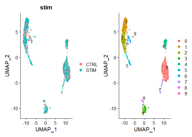
p1 <- DimPlot(immune.combined, reduction = "umap", group.by = "stim")
p1
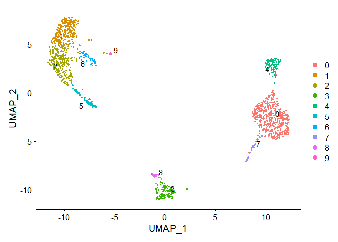
p2 <- DimPlot(immune.combined, reduction = "umap", label = TRUE, repel = TRUE)
p2
p1 + p2
Chapter 2 - Identify conserved cell type markers
# For performing differential expression after integration, we switch back to the original
# data
DefaultAssay(immune.combined) <- "RNA"
nk.markers <- FindConservedMarkers(immune.combined, ident.1 = 6, grouping.var = "stim", verbose = FALSE)

#https://www.biostars.org/p/409790/

#FindMarkers will find markers between two different identity groups - you have to specify both #identity groups. This is useful for comparing the differences between two specific groups.

#FindAllMarkers will find markers differentially expressed in each identity group by comparing #it to all of the others - you don't have to manually define anything. Note that markers may #bleed over between closely-related groups - they are not forced to be specific to only one #group. This is what most people use (and likely what you want).

#FindConservedMarkers will find markers that are conserved between two groups - this can be #useful if you want to find markers that are conserved between a treated and untreated condition #for a specific cell type or group of cells. It means they are differentially expressed compared #to other groups, but have similar expression between the two groups you're actually comparing.

head(nk.markers)
##          CTRL_p_val CTRL_avg_log2FC CTRL_pct.1 CTRL_pct.2 CTRL_p_val_adj
## SNHG12 1.612457e-52        2.255337      0.463      0.017   2.265985e-48
## HSPH1  6.420468e-31        2.951868      0.634      0.088   9.022683e-27
## SCML1  1.689201e-29        2.154189      0.341      0.021   2.373834e-25
## SRSF2  3.068016e-29        2.743712      0.854      0.217   4.311482e-25
## CLK1   4.662395e-27        2.311505      0.585      0.083   6.552063e-23
## NOP58  9.024730e-25        2.290002      0.561      0.081   1.268245e-20
##          STIM_p_val STIM_avg_log2FC STIM_pct.1 STIM_pct.2 STIM_p_val_adj
## SNHG12 9.064908e-32        1.776018      0.292      0.007   1.273892e-27
## HSPH1  5.851049e-11        2.792827      0.542      0.127   8.222480e-07
## SCML1  9.315024e-21        2.278457      0.417      0.034   1.309040e-16
## SRSF2  2.620323e-11        2.535208      0.667      0.186   3.682340e-07
## CLK1   1.253029e-15        2.535546      0.542      0.083   1.760882e-11
## NOP58  1.869061e-15        2.361140      0.583      0.096   2.626592e-11
##            max_pval minimump_p_val
## SNHG12 9.064908e-32   3.224913e-52
## HSPH1  5.851049e-11   1.284094e-30
## SCML1  9.315024e-21   3.378401e-29
## SRSF2  2.620323e-11   6.136031e-29
## CLK1   1.253029e-15   9.324790e-27
## NOP58  1.869061e-15   1.804946e-24
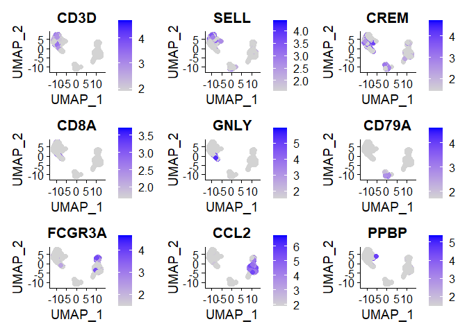
FeaturePlot(immune.combined, features = c("CD3D", "SELL", "CREM", "CD8A", "GNLY", "CD79A", "FCGR3A", "CCL2", "PPBP"), min.cutoff = "q9",pt.size = 2)
 # Chapter 2 - Renaming clusters
levels(immune.combined)
## [1] "0" "1" "2" "3" "4" "5" "6" "7" "8" "9"
renamed.immune.combined <- RenameIdents(immune.combined, "1"= "new 1")
levels(renamed.immune.combined)
##  [1] "new 1" "0"     "2"     "3"     "4"     "5"     "6"     "7"     "8"
## [10] "9"
Chapter 2 - Dimplot with new cluster names
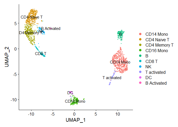
immune.combined <- RenameIdents(immune.combined, "0" = "CD14 Mono", "1" = "CD4 Naive T", "2" = "CD4 Memory T","3" = "CD16 Mono", "4" = "B", "5" = "CD8 T", "6" = "NK", "7" = "T activated", "8" = "DC", "9" = "B Activated", "10" = "Mk", "11" = "pDC", "12" = "Eryth", "13" = "Mono/Mk Doublets", "14" = "HSPC")
## Warning: Cannot find identity 14

## Warning: Cannot find identity 13

## Warning: Cannot find identity 12

## Warning: Cannot find identity 11

## Warning: Cannot find identity 10
levels(immune.combined)
##  [1] "CD14 Mono"    "CD4 Naive T"  "CD4 Memory T" "CD16 Mono"    "B"
##  [6] "CD8 T"        "NK"           "T activated"  "DC"           "B Activated"
table(Idents(object = immune.combined))
##
##    CD14 Mono  CD4 Naive T CD4 Memory T    CD16 Mono            B        CD8 T
##          640          386          356          179          151          111
##           NK  T activated           DC  B Activated
##           65           64           34           14
DimPlot(immune.combined, label = TRUE)
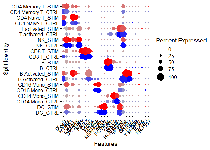
Idents(immune.combined) <- factor(Idents(immune.combined), levels = c("HSPC", "Mono/Mk Doublets","pDC", "Eryth", "Mk", "DC", "CD14 Mono", "CD16 Mono", "B Activated", "B", "CD8 T", "NK", "T activated","CD4 Naive T", "CD4 Memory T"))
markers.to.plot <- c("CD3D", "CREM", "HSPH1", "SELL", "GIMAP5", "CACYBP", "GNLY", "NKG7", "CCL5", "CD8A", "MS4A1", "CD79A", "MIR155HG", "NME1", "FCGR3A", "VMO1", "CCL2", "S100A9", "HLA-DQA1","GPR183", "PPBP", "GNG11", "HBA2", "HBB", "TSPAN13", "IL3RA", "IGJ", "PRSS57")
Chapter 2 - Dotplot
DotPlot(immune.combined, features = markers.to.plot, cols = c("blue", "red"), dot.scale = 8, split.by = "stim") + RotatedAxis()
Chapter 2 - Identify differential expressed genes across conditions
library(ggplot2)
## Warning: package 'ggplot2' was built under R version 4.1.2
library(cowplot)
##
## Attaching package: 'cowplot'

## The following object is masked from 'package:patchwork':
##
##     align_plots
theme_set(theme_cowplot())
t.cells <- subset(immune.combined, idents = "CD4 Naive T")
Idents(t.cells) <- "stim"
avg.t.cells <- as.data.frame(log1p(AverageExpression(t.cells, verbose = FALSE)$RNA))
avg.t.cells$gene <- rownames(avg.t.cells)

cd14.mono <- subset(immune.combined, idents = "CD14 Mono")
Idents(cd14.mono) <- "stim"
avg.cd14.mono <- as.data.frame(log1p(AverageExpression(cd14.mono, verbose = FALSE)$RNA))
avg.cd14.mono$gene <- rownames(avg.cd14.mono)

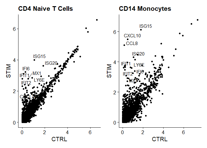
genes.to.label = c("ISG15", "LY6E", "IFI6", "ISG20", "MX1", "IFIT2", "IFIT1", "CXCL10", "CCL8")
p1 <- ggplot(avg.t.cells, aes(CTRL, STIM)) + geom_point() + ggtitle("CD4 Naive T Cells")
p1 <- LabelPoints(plot = p1, points = genes.to.label, repel = TRUE)
## When using repel, set xnudge and ynudge to 0 for optimal results
p2 <- ggplot(avg.cd14.mono, aes(CTRL, STIM)) + geom_point() + ggtitle("CD14 Monocytes")
p2 <- LabelPoints(plot = p2, points = genes.to.label, repel = TRUE)
## When using repel, set xnudge and ynudge to 0 for optimal results
p1 + p2
 # Chapter 2 - Inteferon response
immune.combined$celltype.stim <- paste(Idents(immune.combined), immune.combined$stim, sep = "_")
immune.combined$celltype <- Idents(immune.combined)
Idents(immune.combined) <- "celltype.stim"

b.interferon.response <- FindMarkers(immune.combined, ident.1 = "B_STIM", ident.2 = "B_CTRL", verbose = FALSE)

head(b.interferon.response, n = 15)
##                 p_val avg_log2FC pct.1 pct.2    p_val_adj
## IFIT1    1.166508e-28   4.521337 1.000 0.071 1.639293e-24
## IFIT3    3.708120e-27   3.986884 1.000 0.298 5.211021e-23
## IFITM3   4.715986e-26   2.958064 1.000 0.690 6.627375e-22
## ISG15    4.854345e-26   4.917321 1.000 0.500 6.821811e-22
## ISG20    8.180154e-26   3.478169 1.000 0.464 1.149557e-21
## IFIT2    9.153945e-26   3.319417 1.000 0.214 1.286404e-21
## IFI6     1.108080e-25   3.122246 1.000 0.357 1.557184e-21
## LY6E     1.882624e-25   2.822519 1.000 0.440 2.645651e-21
## APOBEC3A 1.514663e-24   3.352339 1.000 0.452 2.128555e-20
## OASL     1.793719e-24   3.087877 0.955 0.179 2.520713e-20
## CXCL10   7.132351e-24   3.939777 1.000 0.333 1.002309e-19
## MX1      7.954234e-24   3.088767 0.955 0.131 1.117809e-19
## TNFSF10  9.491629e-24   2.687823 1.000 0.512 1.333859e-19
## RSAD2    9.691537e-24   3.354510 0.925 0.119 1.361952e-19
## CXCL11   1.453433e-22   3.924294 0.851 0.036 2.042510e-18
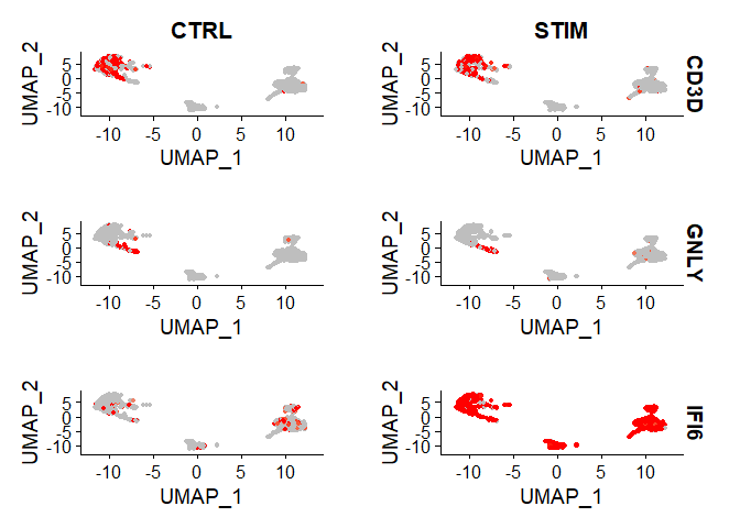
FeaturePlot(immune.combined, features = c("CD3D", "GNLY", "IFI6"), split.by = "stim", max.cutoff = 2, cols = c("grey", "red"))
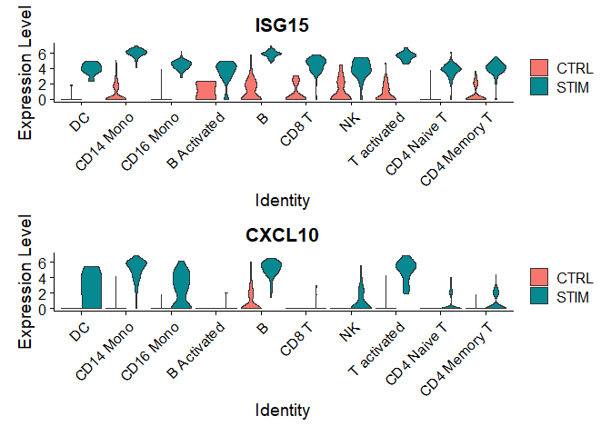
 # Chapter 2 - Violin plot on different conditions
plots <- VlnPlot(immune.combined, features = c("ISG15", "CXCL10"), split.by = "stim", group.by = "celltype", pt.size = 0, combine = FALSE)
## The default behaviour of split.by has changed.
## Separate violin plots are now plotted side-by-side.
## To restore the old behaviour of a single split violin,
## set split.plot = TRUE.
##
## This message will be shown once per session.
wrap_plots(plots = plots, ncol = 1)
